
이번에는 지난 시간에 Knowledge Distillation의 개념에 대해서 알아본 것에 이어서, 파이썬 코딩을 통해서 Knowledge Distillation을 구현해보겠습니다.
1. 파이썬 코드를 통해 구현하는 Knowledge Distillation - MNIST 데이터 분류
- 이번 코드 작성간에는 Knowledge Distillation 구현 간, MNIST 데이터를 활용하여 분류 성능을 확인해보겠습니다.
- MNIST 데이터에 대한 설명은 아래 포스팅을 참조하시면 되겠습니다.
[딥러닝 with 파이썬] GAN (Generative Adversarial Networks) / 생성적 적대 신경망 / MNIST 데이터로 구현
[딥러닝 with 파이썬] GAN (Generative Adversarial Networks) / 생성적 적대 신경망 / MNIST 데이터로 구현
이번에는 GAN, 생성적 적대 신경망에 대해서 알아보겠습니다. 1. GAN이란? - GAN은 Generative Adversarial Network의 약자로, 생성적 적대 신경망으로 불립니다. - 이는 딥러닝을 기반으로 한 모델로서, 이름
jaylala.tistory.com
- 또한, Knowledge Distillation 코드 구현은 아래 Github를 참조했습니다.
** 코드는 Colab에서 실행될 수 있게 작성되어 있습니다.
- 먼저 필요한 라이브러리를 임포트 해줍니다.
|
1
2
3
4
5
6
7
8
9
10
11
12
13
14
15
|
import torch
import torch.nn as nn
import torch.nn.functional as F
import torch.optim as optim
from torchvision import datasets, transforms
import torchvision.models as models
from torch.utils.data import DataLoader
import time
import os
import copy
from torchvision.transforms.functional import to_pil_image
import matplotlib.pyplot as plt
%matplotlib inline
device = torch.device('cuda' if torch.cuda.is_available() else 'cpu')
|
cs |
* Pytorch로 모델을 구현하겠으며, 이미지분류 작업을 위해 파이토치의 CV 패키지인 torchvision을 활용해 데이터로드 및 형태 변형을 하였습니다.
* %matplotlib inline : Jupyter notebook 환경에서 그림을 인라인으로 표시하기 위해 사용
* 컴퓨팅 작업에 gpu 활용하기 위해 cuda를 활용해줍니다.
- MNIST 데이터 셋을 저장하기 위한 디렉토리를 지정합니다.
|
1
2
3
4
5
6
7
8
|
# make directory to save dataset
def createFolder(directory):
try:
if not os.path.exists(directory):
os.makedirs(directory)
except OSerror:
print('Error')
createFolder('./data')
|
cs |
* 위와 같이 지정하게되면, Google Colud 상 '/content/data' 디렉토리에 'data'라는 이름의 폴더가 생성됩니다.
- 이미지 데이터의 전처리를 위해 컴포지션을 정의합니다.
|
1
2
3
4
5
|
# define transformation
ds_transform = transforms.Compose([
transforms.ToTensor(),
transforms.Normalize((0.1307,),(0.3081,))
])
|
cs |
* 먼저 해당 데이터를 'ToTensor'를 활용해 텐서로 만들고
* 데이터의 정규화를 수행합니다. 해당 MNIST 데이터셋 모든 이미지의 픽셀 값 평균은 0.3081이며, 표준편차는 0.1307 이기에 이를 활용하게되면 평균이 0, 표준편차가 1이 되게 만들 수 있습니다.
- 이제 MNIST 데이터를 다운로드 받아줍니다.
|
1
2
3
|
# load MNIST dataset
train_ds = datasets.MNIST('/content/data',train=True, download=True, transform=ds_transform)
val_ds = datasets.MNIST('/content/data',train=False, download=True, transform=ds_transform)
|
cs |
* 해당 데이터셋은 이미 train과 test로 데이터가 분류되어 있으므로, 위와 같은 코드를 활용해 train 데이터는 train_ds로, test 데이터는 val_ds로 저장하며, 위에서 정의한 'ds_transform' 함수를 활용해 Raw data의 전처리(텐서화 -> 표준화)를 진행합니다.
- MNIST 데이터의 샘플 이미지를 확인해보겠습니다.
|
1
2
3
4
5
6
7
8
9
10
11
12
|
# check sample image
for x, y in train_dl:
print(x.shape, y.shape)
break
num = 4
img = x[:num]
plt.figure(figsize=(15,15))
for i in range(num):
plt.subplot(1,num+1,i+1)
plt.imshow(to_pil_image(0.1307*img[i]+0.3081), cmap='gray')
|
cs |
* 확인을 위해서 matplotlib의 imshow 기능을 활용하겠습니다. 이때, ds_transform으로 정규화 되어 있는 데이터를 시각화 하기 위해 앞서 활용한 모든 이미지 데이터의 픽셀 표준편차(0.1307)를 곱해주고 평균(0.3081)을 더해줍니다.
* 이미지는 총 4개를 확인하겠습니다.
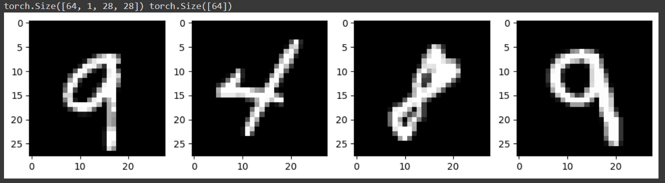
*torch.Size([64,1,28,28]) : 입력 이미지 데이터의 크기를 나타내는 부분입니다. 이는 4차원 텐서를 의미하는데요
64는 미니배치의 크기 / 1은 이미지의 채널 수 (흑백 이므로 1개 채널) / 첫 번째 28은 이미지의 높이 / 두 번째 28은 이미지의 너비를 의미합니다.
* torch.Size([64]) : 미니배치의 정답 레이블의 크기를 나타냅니다.
- 다음은 Knowledge Distilation의 Teacher 클래스를 정의해줍니다. 나중에 정의할 Student 클래스보다 크게 설정합니다.
|
1
2
3
4
5
6
7
8
9
10
11
12
13
14
15
16
17
|
class Teacher(nn.Module):
def __init__(self):
super().__init__()
self.fc1 = nn.Linear(28*28, 1200)
self.bn1 = nn.BatchNorm1d(1200)
self.fc2 = nn.Linear(1200,1200)
self.bn2 = nn.BatchNorm1d(1200)
self.fc3 = nn.Linear(1200, 10)
def forward(self,x):
x = x.view(-1, 28*28)
x = F.relu(self.bn1(self.fc1(x)))
x = F.dropout(x,p=0.8)
x = F.relu(self.bn2(self.fc2(x)))
x = F.dropout(x,p=0.8)
x = self.fc3(x)
return x
|
cs |
* 먼저, Teacher클래스를 neural network로 정의하고 이 클래스에 첫 번째 전 연결층인 fc1은 입력 텐서의 크기가 28*28(MNIST 데이터의 픽셀크기)이고 출력 텐서의 크기는 1200입니다.
* 첫번째 BatchNormalization은 1차원 값에 대해서 실시하며(2차원의 MNIST 데이터가 1차원의 형태로 변형되어 신경망에 들어왔기 때문) 1200개의 텐서를 입력값으로 받고 출력합니다.
* 두번째 전 연결층인 fc2는 입력 1200, 출력 1200 / 두번째 BatchNormalization도 동일하게 1차원 값에 대해 1200개의 텐서를 입력값으로 받고 출력하며
* 마지막 전 연결층인 fc3는 입력 1200, 출력 텐서의 크기는 10입니다. MNIST 데이터는 10개의 클래스(0부터 9까지)를 가지고 있기때문에 위와 같이 설정합니다.
* 이후 forward pass를 정의합니다.
먼저 view 함수를 통해 텐서의 모양을 변경하는데, -1을 활용해 가로 28, 세로 28의 2차원의 형태인 MNIST 데이터를 1차원의 형태로 만듭니다. 이를 조금 더 자세히보면, X라고 하는 텐서를 (?, 28*28)로 바꾸라는 의미이며, MNIST데이터가 2차원이면서 가로 28 세로 28이기때문에
기존 : (28, 28) 을 변경 : (? , 28*28)로 바꾸라는 의미이므로, ? 는 1이 됩니다
* 다시 forward pass 함수에 대해서 알아보면
1) view를 활용한 1차원 텐서로 reshape
2) fc1 레이어로 입력값 전달 후 출력값을 batchnormalization 하고 이 값을 활성화 함수인 relu를 통해 전달
3) 2)에서 전달된 1200개의 노드 중 80%의 레이어를 비활성화 시켜
4) 다음 fc2 레이어에 전달하고, batchnormalizaion 후 relu를 통해 다시 전달
5) 또 다시 전달된 1200개의 노드 중 80%의 레이어를 비활성화시켜
6) 다음 fc2 레이어에 전달하여 최종 10개의 노드의 출력을 도출하는
과정을 보이고 있습니다.
- teacher 모델을 통해 전달된 텐서가 어떤 형태로 바뀌는지 확인해봅니다. (코드가 복잡해지고 길어지면 이러한 출력값들의 텐서 형태가 다른 경우가 종종생깁니다. 확인해보면 나중에 발생할 수 있는 오류를 방지할 수 있습니다)
|
1
2
3
4
5
|
# check
x = torch.randn(16,1,28,28).to(device)
teacher = Teacher().to(device)
output = teacher(x)
print(output.shape)
|
cs |
* x 라는 16개의 미니배치 크기를 가지고, 1개의 채널을 가진, 높이 28 / 너비 28의 랜덤 텐서를 만들고
* 이를 위에서 정의한 teacher 모델에 넣은 뒤
* 결과를 output으로 정의해 출력해보면 아래와 같은 결과가 나오게 됩니다.
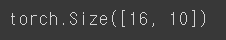
* 출력 텐서는 16개의 미니배치 샘플에 대해 각각의클래스 스코어를 나타내는 10개의 값으로 구성됨을 확인할 수 있습니다. 원하는 결과가 나왔습니다.
- 다음은 정의된 Neural Network 모델의 가중치를 초기화해줍니다.
|
1
2
3
4
5
6
7
8
9
10
11
12
13
|
# weight initialization
def initialize_weights(model):
classname = model.__class__.__name__
# fc layer
if classname.find('Linear') != -1:
nn.init.normal_(model.weight.data, 0.0, 0.02)
nn.init.constant_(model.bias.data, 0)
# batchnorm
elif classname.find('BatchNorm') != -1:
nn.init.normal_(model.weight.data, 1.0, 0.02)
nn.init.constant_(model.bias.data, 0)
teacher.apply(initialize_weights);
|
cs |
* initialize_weights라는 함수를 정의하고 model 객체를 입력으로 받습니다
* model의 클래스 이름을 가져오고
클래스의 이름이 Linear인 경우, 가중치 텐서를 평균은 0.0 / 표준편차는 0.02인 정규분포 값들 중에서 임의로 추출해 만들어주며, 편향 텐서는 0으로 고정해줍니다.
클래스의 이름이 BatchNorm인 경우, 가중치 텐서들을 평균 1.0 / 표준편차는 0.02인 정규분포 값들 중에서 임의로 추출해 만들어주고, 편향 텐서는 0으로 고정해줍니다.
* 이렇게 초기값이 설정된 가중치 및 편향을 teacher class에 정의해줍니다.
- 이제 손실함수와 옵티마이저를 불러옵니다.
|
1
2
3
4
5
6
7
8
9
|
# loss function
loss_func = nn.CrossEntropyLoss()
# optimizer
opt = optim.Adam(teacher.parameters())
# lr scheduler
from torch.optim.lr_scheduler import ReduceLROnPlateau
lr_scheduler = ReduceLROnPlateau(opt, mode='min', factor=0.1, patience=10)
|
cs |
* 이진분류 문제이기때문에 손실함수는 CrossEntropyLoss()로 정해 loss_func 로 정의해주고
* Gradient Descent간 활용할 옵티마이저는 Adam으로 설정하며 teacher class의 parameter / 즉, weight와 bias에 대해 적용하는 것을 정의해줍니다.
* 이후 lr / Learning Rate / 학습률 스케쥴러를 설정하고 초기화해줍니다. 이때 ReduceLROnPlateau 스케쥴러를 사용합니다.
이 스케쥴러는 주로 검증 손실을 모니터링하고 검증 손실이 더이상 개선되지 않을때 학습률을 조절하는데 사용합니다.
이때 opt는 위에서 정의한 옵타미어저인 opt를 사용함을 의미하고,
mode는 손실을 줄이는 방향을 의미하는데 min으로 설정하여 손실을 최소화하는 방향으로 학습률을조절함을 의미하고
factor는 학습률을 줄일 때 사용할 인수로, factor=0.1 이라는 의미는 손실이 개선되지 않을 때 학습률을 10%씩 줄여간다는 의미를 말합니다.
patience는 개선되지 않는 에포크의 수를 의미하며 위의 factor와 연관되어 있습니다. 즉, 위에서 지정한 10을 바탕으로 해석해보면 10번 연속으로 loss가 줄어들지 않으면 학습률을 10%감소하여 적용한다는 의미가 되겠습니다.
- 모델의 훈련 및 검증을 수행하는 함수들을 정의합니다.
|
1
2
3
4
5
6
7
8
9
10
11
12
13
14
15
16
17
18
19
20
21
22
23
24
25
26
27
28
29
30
31
32
33
34
35
36
37
38
39
40
41
42
43
44
45
46
47
48
49
50
51
52
53
54
55
56
57
58
59
60
61
62
63
64
65
66
67
68
69
70
71
72
73
74
75
76
77
78
79
80
81
82
83
84
85
86
87
88
89
90
91
92
93
94
95
96
97
98
99
100
101
|
# get current lr
def get_lr(opt):
for param_group in opt.param_groups:
return param_group['lr']
# calculate the metric per mini-batch
def metric_batch(output, target):
pred = output.argmax(1, keepdim=True)
corrects = pred.eq(target.view_as(pred)).sum().item()
return corrects
# calculate the loss per mini-batch
def loss_batch(loss_func, output, target, opt=None):
loss_b = loss_func(output, target)
metric_b = metric_batch(output, target)
if opt is not None:
opt.zero_grad()
loss_b.backward()
opt.step()
return loss_b.item(), metric_b
# calculate the loss per epochs
def loss_epoch(model, loss_func, dataset_dl, sanity_check=False, opt=None):
running_loss = 0.0
running_metric = 0.0
len_data = len(dataset_dl.dataset)
for xb, yb in dataset_dl:
xb = xb.to(device)
yb = yb.to(device)
output = model(xb)
loss_b, metric_b = loss_batch(loss_func, output, yb, opt)
running_loss += loss_b
if metric_b is not None:
running_metric += metric_b
if sanity_check is True:
break
loss = running_loss / len_data
metric = running_metric / len_data
return loss, metric
# function to start training
def train_val(model, params):
num_epochs=params['num_epochs']
loss_func=params['loss_func']
opt=params['optimizer']
train_dl=params['train_dl']
val_dl=params['val_dl']
sanity_check=params['sanity_check']
lr_scheduler=params['lr_scheduler']
path2weights=params['path2weights']
loss_history = {'train': [], 'val': []}
metric_history = {'train': [], 'val': []}
best_loss = float('inf')
best_model_wts = copy.deepcopy(model.state_dict())
start_time = time.time()
for epoch in range(num_epochs):
current_lr = get_lr(opt)
print('Epoch {}/{}, current lr= {}'.format(epoch, num_epochs-1, current_lr))
model.train()
train_loss, train_metric = loss_epoch(model, loss_func, train_dl, sanity_check, opt)
loss_history['train'].append(train_loss)
metric_history['train'].append(train_metric)
model.eval()
with torch.no_grad():
val_loss, val_metric = loss_epoch(model, loss_func, val_dl, sanity_check)
loss_history['val'].append(val_loss)
metric_history['val'].append(val_metric)
if val_loss < best_loss:
best_loss = val_loss
best_model_wts = copy.deepcopy(model.state_dict())
torch.save(model.state_dict(), path2weights)
print('Copied best model weights!')
lr_scheduler.step(val_loss)
if current_lr != get_lr(opt):
print('Loading best model weights!')
model.load_state_dict(best_model_wts)
print('train loss: %.6f, val loss: %.6f, accuracy: %.2f, time: %.4f min' %(train_loss, val_loss, 100*val_metric, (time.time()-start_time)/60))
print('-'*10)
model.load_state_dict(best_model_wts)
return model, loss_history, metric_history
|
cs |
* get_lr(opt): 주어진 옵티마이저(opt)에서 현재 학습률을 가져오는 함수입니다.
* metric_batch(output, target): 미니배치 단위로 예측 결과(output)와 실제 타겟(target)을 비교하여 정확도를 계산하는 함수입니다. 미니배치 내에서 올바르게 분류된 샘플 수를 반환합니다.
* loss_batch(loss_func, output, target, opt=None): 미니배치 단위로 손실(loss_b) 및 정확도(metric_b)를 계산하고, 필요한 경우 옵티마이저(opt)를 사용하여 역전파 및 가중치 업데이트를 수행합니다.
* loss_epoch(model, loss_func, dataset_dl, sanity_check=False, opt=None): 에포크 단위로 손실(loss) 및 정확도(metric)를 계산하는 함수입니다. sanity_check가 활성화되면 일부 미니배치만 처리합니다.
* train_val(model, params): 모델 훈련 및 검증을 수행하는 함수로, 주요 훈련 루프를 제공합니다. 설정 및 하이퍼파라미터(params)에 따라 모델을 훈련하고, 최적의 모델 가중치를 저장합니다. 또한, 학습률 스케줄링과 관련된 작업도 수행합니다.
- 이제 최종적으로 모델에 활용할 하이퍼 파라미터를 정의합니다.
|
1
2
3
4
5
6
7
8
9
10
11
12
13
|
# set hyper parameters
params_train = {
'num_epochs':30,
'optimizer':opt,
'loss_func':loss_func,
'train_dl':train_dl,
'val_dl':val_dl,
'sanity_check':False,
'lr_scheduler':lr_scheduler,
'path2weights':'./models/teacher_weights.pt',
}
createFolder('./models')
|
cs |
* 학습 회수는 30회
* 옵티마이저, 손실함수, train 데이터, validation 데이터, lr scheduler는 위에서 정의한 함수를 활용하고
sanity_check 는 미니배치의 테스트 모드를 활성화할지 여부인데 비활성화시키고
학습간 생성되는 모델의 가중치는 위 경로에 저장하며, 이를 위해 models라는 폴더를 만들어줍니다.
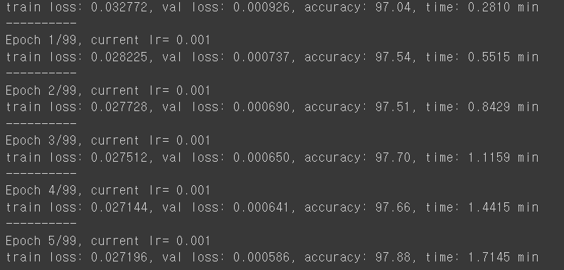
- 이제 정의된 함수들을 바탕으로 학습을 진행해줍니다.
|
1
|
teacher, loss_hist, metric_hist = train_val(teacher, params_train)
|
cs |
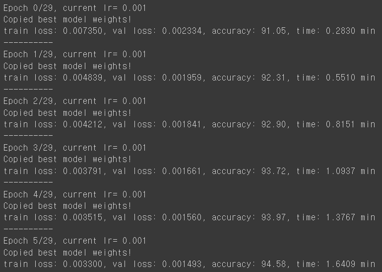
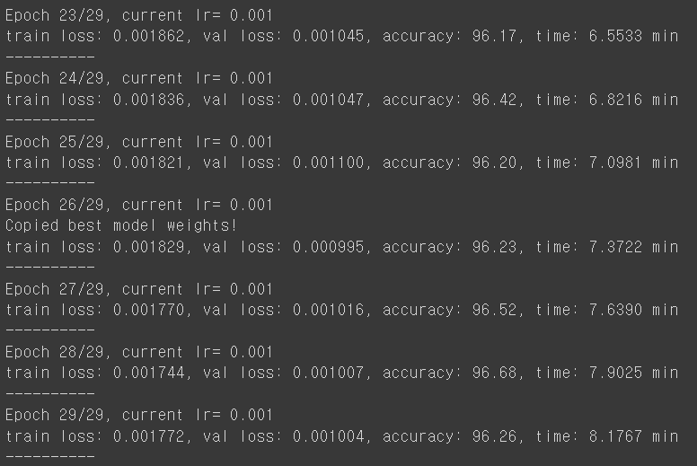
* 중간과정이 일부 생략된 결과이며 30번의 학습을 통해서, 총 8분 가량이 걸렸고 학습된 모델로 검증 데이터를 검증한 결과는, 최초 91%의 정확도에서 96%의 정확도까지 향상된 것을 알 수 있습니다.
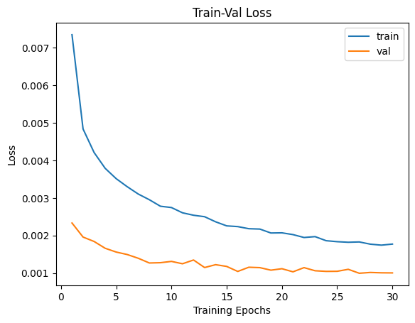
- 이 결과를 시각화해보겠습니다.
|
1
2
3
4
5
6
7
8
9
10
11
12
13
14
15
16
17
18
19
|
num_epochs = params_train['num_epochs']
# Plot train-val loss
plt.title('Train-Val Loss')
plt.plot(range(1, num_epochs+1), loss_hist['train'], label='train')
plt.plot(range(1, num_epochs+1), loss_hist['val'], label='val')
plt.ylabel('Loss')
plt.xlabel('Training Epochs')
plt.legend()
plt.show()
# plot train-val accuracy
plt.title('Train-Val Accuracy')
plt.plot(range(1, num_epochs+1), metric_hist['train'], label='train')
plt.plot(range(1, num_epochs+1), metric_hist['val'], label='val')
plt.ylabel('Accuracy')
plt.xlabel('Training Epochs')
plt.legend()
plt.show()
|
cs |

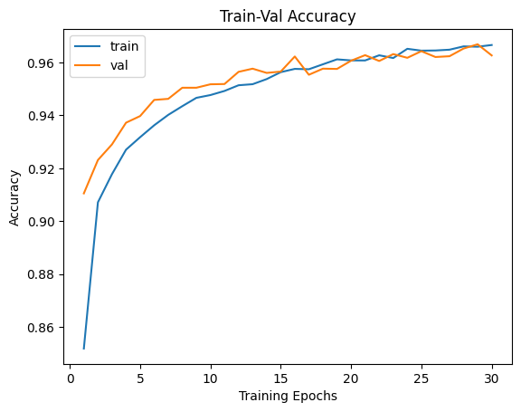
* 아직 train 데이터에 대한 Over fitting이 일어나지는 않았지만 학습률이 둔화되고 있음을 확인할 수 있습니다.
- 이제 Studnet Class를 정의하겠습니다.
|
1
2
3
4
5
6
7
8
9
10
11
12
13
14
15
|
class Student(nn.Module):
def __init__(self):
super().__init__()
self.fc1 = nn.Linear(28*28, 800)
self.bn1 = nn.BatchNorm1d(800)
self.fc2 = nn.Linear(800,800)
self.bn2 = nn.BatchNorm1d(800)
self.fc3 = nn.Linear(800,10)
def forward(self, x):
x = x.view(-1, 28*28)
x = F.relu(self.bn1(self.fc1(x)))
x = F.relu(self.bn2(self.fc2(x)))
x = self.fc3(x)
return x
|
cs |
* Teacher 클래스와 유사하게 정의하였으며, 다른점은 800개의 노드를 사용한다는 점입니다. Teacher 클래스는 1200개의 노드를 사용했던 점과 비교했을때 경량화 되었습니다.
- Student Class의 출력 결과물의 텐서 사이즈를 확인해봅니다.
|
1
2
3
4
5
|
# check
x = torch.randn(16,1,28,28).to(device)
student = Student().to(device)
output = student(x)
print(output.shape)
|
cs |
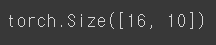
* Teacher Class와 마찬가지로 16개의 미니배치의 크기이며 10개의 클래스가 도출됩니다. Teacher Class의 Soft target에 의해 지도 받기에 이상없습니다.
- teacher 클래스와 유사한 방식으로 weight 및 bias를 초기화해줍니다.
|
1
2
3
4
5
6
7
8
9
10
11
12
13
|
# weight initialization
def initialize_weights(model):
classname = model.__class__.__name__
# fc layer
if classname.find('Linear') != -1:
nn.init.normal_(model.weight.data, 0.0, 0.02)
nn.init.constant_(model.bias.data, 0)
# batchnorm
elif classname.find('BatchNorm') != -1:
nn.init.normal_(model.weight.data, 1.0, 0.02)
nn.init.constant_(model.bias.data, 0)
student.apply(initialize_weights);
|
cs |
- distillation을 위해 학습된 Teacher 모델을 불러오고, Student 모델도 학습 준비를 합니다.
|
1
2
3
4
5
6
7
8
|
teacher = Teacher().to(device)
# load weight
teacher.load_state_dict(torch.load('/content/models/teacher_weights.pt'))
student = Student().to(device)
# optimizer
opt = optim.Adam(student.parameters())
|
cs |
- Total Loss를 정의합니다. 지난 시간에 알아봤던 것처럼 Knowledge Distillation Loss와 Classification Loss를 정의하며 손실 가중치 매개변수인 alpha를 활용하여 최종정의합니다.
|
1
2
3
4
5
6
7
8
9
10
|
# knowledge distillation loss
def distillation(y, labels, teacher_scores, T, alpha):
# distillation loss + classification loss
# y: student
# labels: hard label
# teacher_scores: soft label
return nn.KLDivLoss()(F.log_softmax(y/T), F.softmax(teacher_scores/T)) * (T*T * 2.0 + alpha) + F.cross_entropy(y,labels) * (1.-alpha)
# val loss
loss_func = nn.CrossEntropyLoss()
|
cs |
[딥러닝 with 파이썬] Knowledge Distillation이란? 딥러닝 모델의 지식 증류기법이란? (1/2)
- 이제 위에서 정의된 두 손실을 바탕으로 최종 손실을 정의하고 이때 들어가는 T 값 및 Alphar값을 정해서 입력해줍니다. 각 미니 배치에 대한 손실을 계산하고 최적화를 수행하는 함수를 정의합니다.
|
1
2
3
4
5
6
7
8
9
10
|
def distill_loss_batch(output, target, teacher_output, loss_fn=distillation, opt=opt):
loss_b = loss_fn(output, target, teacher_output, T=20.0, alpha=0.7)
metric_b = metric_batch(output, target)
if opt is not None:
opt.zero_grad()
loss_b.backward()
opt.step()
return loss_b.item(), metric_b
|
cs |
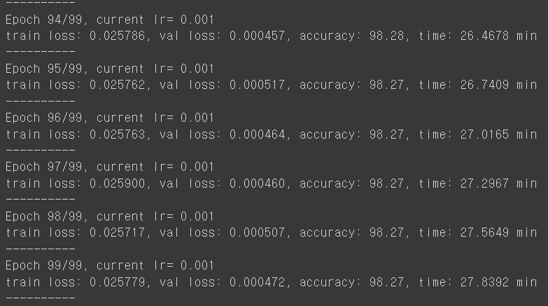
- 이제 학습을 진행하고 결과를 확인합니다.
|
1
2
3
4
5
6
7
8
9
10
11
12
13
14
15
16
17
18
19
20
21
22
23
24
25
26
27
28
29
30
31
32
33
34
35
36
37
38
39
40
41
42
43
44
45
46
|
num_epochs= 100
loss_history = {'train': [], 'val': []}
metric_history = {'train': [], 'val': []}
best_loss = float('inf')
start_time = time.time()
for epoch in range(num_epochs):
current_lr = get_lr(opt)
print('Epoch {}/{}, current lr= {}'.format(epoch, num_epochs-1, current_lr))
# train
student.train()
running_loss = 0.0
running_metric = 0.0
len_data = len(train_dl.dataset)
for xb, yb in train_dl:
xb = xb.to(device)
yb = yb.to(device)
output = student(xb)
teacher_output = teacher(xb).detach()
loss_b, metric_b = distill_loss_batch(output, yb, teacher_output, loss_fn=distillation, opt=opt)
running_loss += loss_b
running_metric_b = metric_b
train_loss = running_loss / len_data
train_metric = running_metric / len_data
loss_history['train'].append(train_loss)
metric_history['train'].append(train_metric)
# validation
student.eval()
with torch.no_grad():
val_loss, val_metric = loss_epoch(student, loss_func, val_dl)
loss_history['val'].append(val_loss)
metric_history['val'].append(val_metric)
lr_scheduler.step(val_loss)
print('train loss: %.6f, val loss: %.6f, accuracy: %.2f, time: %.4f min' %(train_loss, val_loss, 100*val_metric, (time.time()-start_time)/60))
print('-'*10)
|
cs |
|
1
2
3
4
5
6
7
8
9
10
11
12
13
14
15
16
17
18
|
# Plot train-val loss
plt.title('Train-Val Loss')
num_epochs = len(loss_hist['train']) # 에포크 수를 기준으로 x 축 설정
plt.plot(range(1, num_epochs+1), loss_hist['train'], label='train')
plt.plot(range(1, num_epochs+1), loss_hist['val'], label='val')
plt.ylabel('Loss')
plt.xlabel('Training Epochs')
plt.legend()
plt.show()
# plot train-val accuracy
plt.title('Train-Val Accuracy')
plt.plot(range(1, num_epochs+1), metric_hist['train'], label='train')
plt.plot(range(1, num_epochs+1), metric_hist['val'], label='val')
plt.ylabel('Accuracy')
plt.xlabel('Training Epochs')
plt.legend()
plt.show()
|
cs |

* Student 모델이 Teacher 모델의 지도를 받아 최초학습부터 더 좋은 성과를 보여주며, 최종적으로도 2%이상 향상된 정확도를 보여주었습니다.
더 가벼운 모델임에도 선생님의 지도를 받아 학생이 더 좋은 결과물을 만들어 냈습니다.


댓글