[딥러닝 with Python] 변이형 오토인코더(Variational Auto Encoder) 추가본 - CelebA Faces 활용

[해당 포스팅은 "만들면서 배우는 생성 AI 2탄" 을 참조했습니다]

 

이번 지난번 2편의 변이형 오토 인코더에 대한 포스팅의 확장 버전입니다.

[생성 AI] 변이형 오토인코더(Variational Auto Encoder) (1/2)

[생성 AI] 변이형 오토인코더(Variational Auto Encoder) (1/2)

[생성 AI] 변이형 오토인코더(Variational Auto Encoder) (2/2)

[생성 AI] 변이형 오토인코더(Variational Auto Encoder) (2/2)

 

 

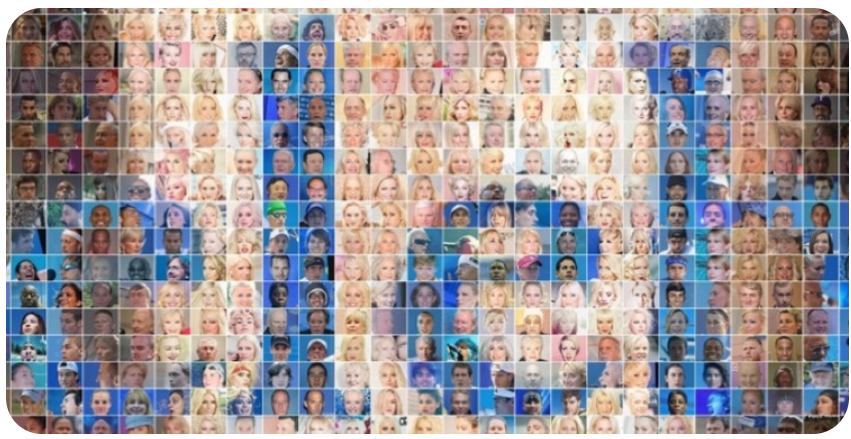
이번에는 CelebA Faces 데이터를 활용해서 변이형 오토 인코더를 구현해보겠습니다.

 

먼저, CelebA Faces 데이터에 대해서 알아보겠습니다.

 

CelebA Faces 데이터 셋의 특징은 아래와 같습니다.

1) 데이터의 개수 : 202,599개

2) 포함된 사람의 수 : 10,177명

 * 1명당 약 20개의 사진이 있다고 보면 됨

 * 사람의 이름에 대한 레이블은 주어지지 않았음

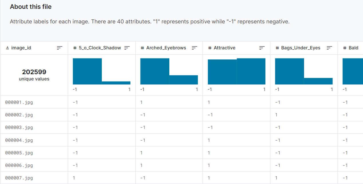
3) 각 얼굴에 대해서는 40개의 이진 레이블(Binary Label)이 있음. 

 * 아래 그림과 같이 다양한 attributes에 대해서 1 또는 -1로 레이블 되어 있습니다. 자세한 사항은 아래에 있는 kaggle 주소에 들어가셔서 참조하시면 되겠습니다.

 

 

CelebA 데이터 출처 : 캐글(kaggle)

https://www.kaggle.com/datasets/jessicali9530/celeba-dataset

CelebFaces Attributes (CelebA) Dataset

 

 

이제 이 데이터를 활용해 변이형 오토 인코더를 구현해보겠습니다. 

 

 

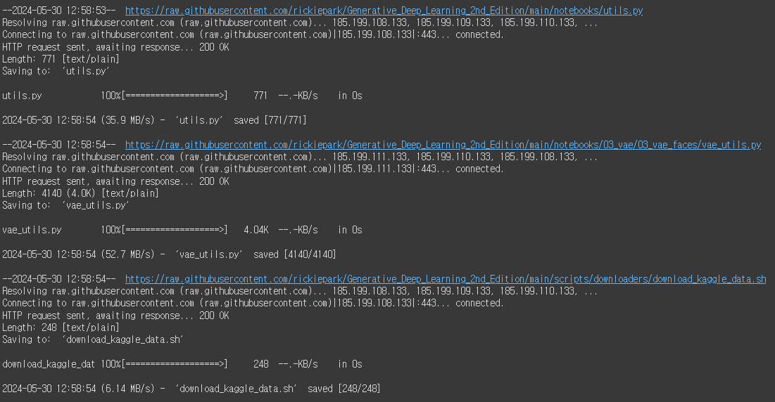
먼저, 해당 깃허브에서 VAE 구현에 활용한 유틸 파일과 kaggle에서 해당 데이터를 가져와줍니다.

import sys

# 코랩의 경우 깃허브 저장소로부터 utils.py와 vae_utils.py, download_kaggle_data.sh를 다운로드 합니다.

if 'google.colab' in sys.modules:

    !wget https://raw.githubusercontent.com/rickiepark/Generative_Deep_Learning_2nd_Edition/main/notebooks/utils.py

    !mkdir -p notebooks

    !mv utils.py notebooks

    !wget https://raw.githubusercontent.com/rickiepark/Generative_Deep_Learning_2nd_Edition/main/notebooks/03_vae/03_vae_faces/vae_utils.py

    !wget https://raw.githubusercontent.com/rickiepark/Generative_Deep_Learning_2nd_Edition/main/scripts/downloaders/download_kaggle_data.sh

 

 

다음은 변이형 오토인코더 구현에 필요한 라이브러리를 불러와줍니다.

import numpy as np

import matplotlib.pyplot as plt

import tensorflow as tf

import tensorflow.keras.backend as K

from tensorflow.keras import (

    layers,

    models,

    callbacks,

    utils,

    metrics,

    losses,

    optimizers,

)

from scipy.stats import norm

import pandas as pd

from notebooks.utils import sample_batch, display

from vae_utils import get_vector_from_label, add_vector_to_images, morph_faces

 

 

학습에 사용할 하이퍼 파라미터를 정의해줍니다.

IMAGE_SIZE = 64

CHANNELS = 3

BATCH_SIZE = 128

NUM_FEATURES = 64

Z_DIM = 200

LEARNING_RATE = 0.0005

EPOCHS = 10

BETA = 2000

LOAD_MODEL = False

 

 

이제 데이터를 다운로드해줍니다. 

# 코랩일 경우 노트북에서 celeba 데이터셋을 받습니다.

if 'google.colab' in sys.modules:

    # 캐글-->Setttings-->API-->Create New Token에서

    # kaggle.json 파일을 만들어 코랩에 업로드하세요.

    # from google.colab import files

    # files.upload()

    # !mkdir ~/.kaggle

    # !cp kaggle.json ~/.kaggle/

    # !chmod 600 ~/.kaggle/kaggle.json

    # celeba 데이터셋을 다운로드하고 압축을 해제합니다.

    # !kaggle datasets download -d jessicali9530/celeba-dataset

    # !unzip -q celeba-dataset.zip

    #

    # 캐글에서 다운로드가 안 될 경우 역자의 드라이브에서 다운로드할 수 있습니다.

    import gdown

    gdown.download(id='15gJhiDBkltMQz3T97xG-fO4gXTKAWkSB', output='img_align_celeba.zip')

    !unzip -q img_align_celeba.zip

    #

    # output 디렉토리를 만듭니다.

    !mkdir output

 

 

 

이제 다운로드 된 데이터를 로드해줍니다.

# 데이터 로드

train_data = utils.image_dataset_from_directory(

    "./img_align_celeba/img_align_celeba",

    labels=None,

    color_mode="rgb",

    image_size=(IMAGE_SIZE, IMAGE_SIZE),

    batch_size=BATCH_SIZE,

    shuffle=True,

    seed=42,

    interpolation="bilinear",

)

 

 

이제 데이터를 학습 간 효율성 있게 활용하기 위해 전처리를 진행해줍니다. 

0~255의 픽셀 강도를 가지고 있으므로 255로 나누어서 그 범위를 0 ~ 1 로 변형해줍니다.

# 데이터 전처리

def preprocess(img):

    img = tf.cast(img, "float32") / 255.0

    return img

train = train_data.map(lambda x: preprocess(x))

 

 

train 용으로 분리한 데이터의 일부를 가져와서 시각화해줘봅니다.

train_sample = sample_batch(train)

# 훈련 세트의 일부 얼굴 표시

display(train_sample, cmap=None)

 

 

이제 Variational Auto Encoder 함수를 정의해줍니다.

재매개변수화(Reparametrization) 트릭을 구현한 Sampling을 진행해줍니다.

* 즉 잠재 변수인 z를 샘플링하는 것입니다. 이 z 는  (평균 : z_mean, 분산 : exp(z_log_var)) 을 따르는 정규분포에서 샘플링됩니다.

class Sampling(layers.Layer):

    def call(self, inputs):

        z_mean, z_log_var = inputs

        batch = tf.shape(z_mean)[0]

        dim = tf.shape(z_mean)[1]

        epsilon = K.random_normal(shape=(batch, dim))

        return z_mean + tf.exp(0.5 * z_log_var) * epsilon

 

 

다음은 Input 데이터를 활용하여 잠재 변수를 도출하기 위해 인코더(Encoder) 부분을 정의해줍니다.

3x3 Conv(Stirde 2 까지 추가)를 거쳐서 맵의 크기를 줄이고 Channel 수를 늘린 뒤, Batch Normalization과 LeakyReLU를 통해 안정성과 비선형성을 더해줍니다.  특히 LeakyReLU를 통해 Input 값이 음수 영역으로 들어오더라도 작은 기울기를 유지해 Gradient Vanishing 문제를 해결해줍니다. 

* 이때 Flatten은 잠재변수인 z를 생성하기 위해 연결된 것이며, 나중에 디코더에서 인코더와 동일한 구조를 유지하기 위해 마지막 Conv BN LeakyReLU의 결과를 저장해서 디코더를 사용할 때 활용해줍니다.

# 인코더

encoder_input = layers.Input(

    shape=(IMAGE_SIZE, IMAGE_SIZE, CHANNELS), name="encoder_input"

)

x = layers.Conv2D(NUM_FEATURES, kernel_size=3, strides=2, padding="same")(

    encoder_input

)

x = layers.BatchNormalization()(x)

x = layers.LeakyReLU()(x)

x = layers.Conv2D(NUM_FEATURES, kernel_size=3, strides=2, padding="same")(x)

x = layers.BatchNormalization()(x)

x = layers.LeakyReLU()(x)

x = layers.Conv2D(NUM_FEATURES, kernel_size=3, strides=2, padding="same")(x)

x = layers.BatchNormalization()(x)

x = layers.LeakyReLU()(x)

x = layers.Conv2D(NUM_FEATURES, kernel_size=3, strides=2, padding="same")(x)

x = layers.BatchNormalization()(x)

x = layers.LeakyReLU()(x)

x = layers.Conv2D(NUM_FEATURES, kernel_size=3, strides=2, padding="same")(x)

x = layers.BatchNormalization()(x)

x = layers.LeakyReLU()(x)

shape_before_flattening = K.int_shape(x)[1:]  # 디코더에 필요합니다!

x = layers.Flatten()(x)

z_mean = layers.Dense(Z_DIM, name="z_mean")(x)

z_log_var = layers.Dense(Z_DIM, name="z_log_var")(x)

z = Sampling()([z_mean, z_log_var])

encoder = models.Model(encoder_input, [z_mean, z_log_var, z], name="encoder")

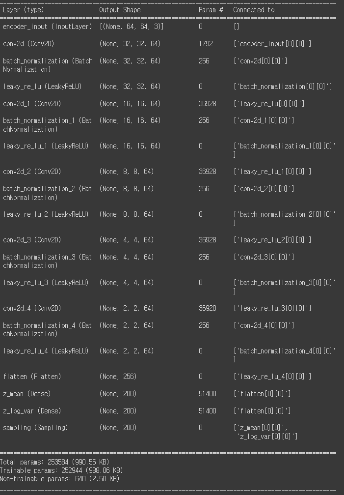
encoder.summary()

 

이와 같은 블록의 연속을 통해서 최종적으로  나온 인코더 모델의 구조는 아래와 같습니다.

* 결과를 보시면 최종 블록의 크기는 2x2에 64개의 채널로 변형되며, 이는 Flatten 되어 256개 ( 2x 2x 64)의 노드로 변형되어 z_mean과 z_log_var 계산에 활용됩니다. 

 

 

다음은 디코더 부분입니다. 디코더의 구조는 인코더의 역방향과 같습니다.

# 디코더

decoder_input = layers.Input(shape=(Z_DIM,), name="decoder_input")

x = layers.Dense(np.prod(shape_before_flattening))(decoder_input)

x = layers.BatchNormalization()(x)

x = layers.LeakyReLU()(x)

x = layers.Reshape(shape_before_flattening)(x)

x = layers.Conv2DTranspose(

    NUM_FEATURES, kernel_size=3, strides=2, padding="same"

)(x)

x = layers.BatchNormalization()(x)

x = layers.LeakyReLU()(x)

x = layers.Conv2DTranspose(

    NUM_FEATURES, kernel_size=3, strides=2, padding="same"

)(x)

x = layers.BatchNormalization()(x)

x = layers.LeakyReLU()(x)

x = layers.Conv2DTranspose(

    NUM_FEATURES, kernel_size=3, strides=2, padding="same"

)(x)

x = layers.BatchNormalization()(x)

x = layers.LeakyReLU()(x)

x = layers.Conv2DTranspose(

    NUM_FEATURES, kernel_size=3, strides=2, padding="same"

)(x)

x = layers.BatchNormalization()(x)

x = layers.LeakyReLU()(x)

x = layers.Conv2DTranspose(

    NUM_FEATURES, kernel_size=3, strides=2, padding="same"

)(x)

x = layers.BatchNormalization()(x)

x = layers.LeakyReLU()(x)

decoder_output = layers.Conv2DTranspose(

    CHANNELS, kernel_size=3, strides=1, activation="sigmoid", padding="same"

)(x)

decoder = models.Model(decoder_input, decoder_output)

decoder.summary()

 

 

 

자 이제 이렇게 정의한 인코더와 디코더, 그리고 최초에 불러온 utlis.py 등을 활용해서 최종적인 VAE 함수를 정의해줍니다.

class VAE(models.Model):

    def __init__(self, encoder, decoder, **kwargs):

        super(VAE, self).__init__(**kwargs)

        self.encoder = encoder

        self.decoder = decoder

        self.total_loss_tracker = metrics.Mean(name="total_loss")

        self.reconstruction_loss_tracker = metrics.Mean(

            name="reconstruction_loss"

        )

        self.kl_loss_tracker = metrics.Mean(name="kl_loss")

    @property

    def metrics(self):

        return [

            self.total_loss_tracker,

            self.reconstruction_loss_tracker,

            self.kl_loss_tracker,

        ]

    def call(self, inputs):

        """특정 입력에서 모델을 호출합니다."""

        z_mean, z_log_var, z = encoder(inputs)

        reconstruction = decoder(z)

        return z_mean, z_log_var, reconstruction

    def train_step(self, data):

        """훈련 스텝을 실행합니다."""

        with tf.GradientTape() as tape:

            z_mean, z_log_var, reconstruction = self(data, training=True)

            reconstruction_loss = tf.reduce_mean(

                BETA * losses.mean_squared_error(data, reconstruction)

            )

            kl_loss = tf.reduce_mean(

                tf.reduce_sum(

                    -0.5

                    * (1 + z_log_var - tf.square(z_mean) - tf.exp(z_log_var)),

                    axis=1,

                )

            )

            total_loss = reconstruction_loss + kl_loss

        grads = tape.gradient(total_loss, self.trainable_weights)

        self.optimizer.apply_gradients(zip(grads, self.trainable_weights))

        self.total_loss_tracker.update_state(total_loss)

        self.reconstruction_loss_tracker.update_state(reconstruction_loss)

        self.kl_loss_tracker.update_state(kl_loss)

        return {

            "loss": self.total_loss_tracker.result(),

            "reconstruction_loss": self.reconstruction_loss_tracker.result(),

            "kl_loss": self.kl_loss_tracker.result(),

        }

    def test_step(self, data):

        """검증 스텝을 실행합니다."""

        if isinstance(data, tuple):

            data = data[0]

        z_mean, z_log_var, reconstruction = self(data)

        reconstruction_loss = tf.reduce_mean(

            BETA * losses.mean_squared_error(data, reconstruction)

        )

        kl_loss = tf.reduce_mean(

            tf.reduce_sum(

                -0.5 * (1 + z_log_var - tf.square(z_mean) - tf.exp(z_log_var)),

                axis=1,

            )

        )

        total_loss = reconstruction_loss + kl_loss

        return {

            "loss": total_loss,

            "reconstruction_loss": reconstruction_loss,

            "kl_loss": kl_loss,

        }

    def get_config(self):

        return {}

 

이제 vae 함수를 인스턴스화해줍니다.

# 변이형 오토인코더 생성

vae = VAE(encoder, decoder)

 

 

 

이제 훈련을 진행하기 위한 준비를 합니다.

먼저, 옵티마이저를 위에서 정의한 하이퍼 파라미터를 활용해서 정의해줍니다.

# 변이형 오토인코더 컴파일

optimizer = optimizers.Adam(learning_rate=LEARNING_RATE)

vae.compile(optimizer=optimizer)

 

 

이제 모델의 저장할 체크포인트를 생성해줍니다.

# 모델 저장 체크포인트 생성

model_checkpoint_callback = callbacks.ModelCheckpoint(

    filepath="./checkpoint",

    save_weights_only=False,

    save_freq="epoch",

    monitor="loss",

    mode="min",

    save_best_only=True,

    verbose=0,

)

tensorboard_callback = callbacks.TensorBoard(log_dir="./logs")

class ImageGenerator(callbacks.Callback):

    def __init__(self, num_img, latent_dim):

        self.num_img = num_img

        self.latent_dim = latent_dim

    def on_epoch_end(self, epoch, logs=None):

        random_latent_vectors = tf.random.normal(

            shape=(self.num_img, self.latent_dim)

        )

        generated_images = self.model.decoder(random_latent_vectors)

        generated_images *= 255

        generated_images.numpy()

        for i in range(self.num_img):

            img = utils.array_to_img(generated_images[i])

            img.save("./output/generated_img_%03d_%d.png" % (epoch, i))

 

# 필요한 경우 이전 가중치 로드

if LOAD_MODEL:

    vae.load_weights("./models/vae")

    tmp = vae.predict(train.take(1))

 

 

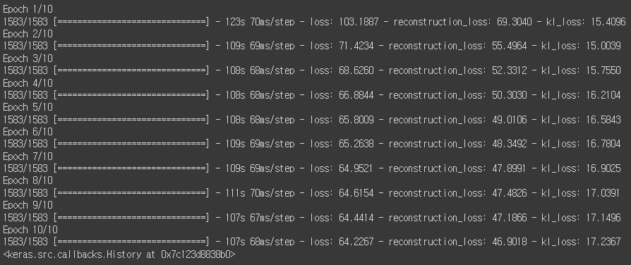
이제 정의한 모델을 피팅하여 학습을 진행해줍니다.

vae.fit(

    train,

    epochs=EPOCHS,

    callbacks=[

        model_checkpoint_callback,

        tensorboard_callback,

        ImageGenerator(num_img=10, latent_dim=Z_DIM),

    ],

)

 

학습된 모델을 저장해줍니다. vae 모델 전체, 그리고 학습된 인코더와 디코더 모두를 저장해줍니다.

# 최종 모델 저장

vae.save("./models/vae")

encoder.save("./models/encoder")

decoder.save("./models/decoder")

 

 

자 이제, 테스트 데이터에서 일부를 선택해서 학습된 vae를 활용해 재구성된 이미지를 확인해봅니다.

# 테스트 세트에서 일부분을 선택합니다.

batches_to_predict = 1

example_images = np.array(

    list(train.take(batches_to_predict).get_single_element())

)

# 오토인코더 예측을 생성하고 출력합니다.

z_mean, z_log_var, reconstructions = vae.predict(example_images)

print("실제 얼굴")

display(example_images)

print("재구성")

display(reconstructions)

 

재구성된 결과는 원본과는 사뭇 달라졌음을 알 수 있습니다. 성별이 바뀐 데이터도 존재하고 특히나 이미지 주변 부분이 Smoothing 해지는 결과를 보이고 있습니다.

 

 

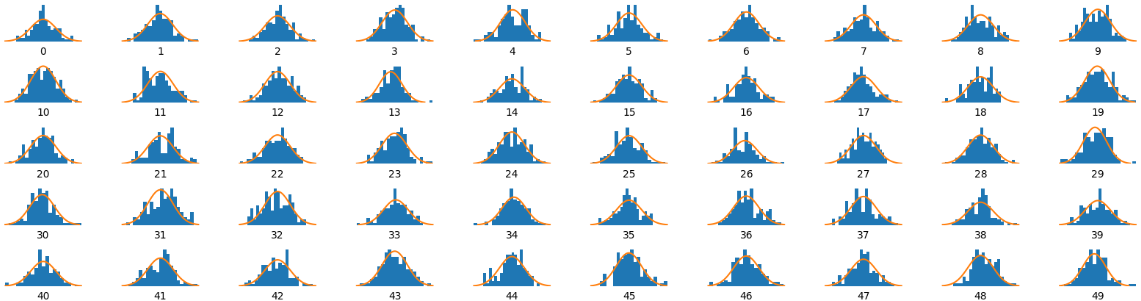
이제 VAE를 사용해 학습 데이터에서 추출한 잠재 변수 z의 분포를 시각화해보겠습니다.

총 200개의 차원으로 저장된 잠재변수 중 50개만을 시각화 해보겠습니다.

_, _, z = vae.encoder.predict(example_images)

x = np.linspace(-3, 3, 100)

fig = plt.figure(figsize=(20, 5))

fig.subplots_adjust(hspace=0.6, wspace=0.4)

for i in range(50):

    ax = fig.add_subplot(5, 10, i + 1)

    ax.hist(z[:, i], density=True, bins=20)

    ax.axis("off")

    ax.text(

        0.5, -0.35, str(i), fontsize=10, ha="center", transform=ax.transAxes

    )

    ax.plot(x, norm.pdf(x))

plt.show()

 

시각화 결과, 총 50개의 잠재 변수 대부분 정규성을 보이는 것을 확인할 수 있습니다. 학습이 비교적 잘 이루어 진 것 같습니다.

 

 

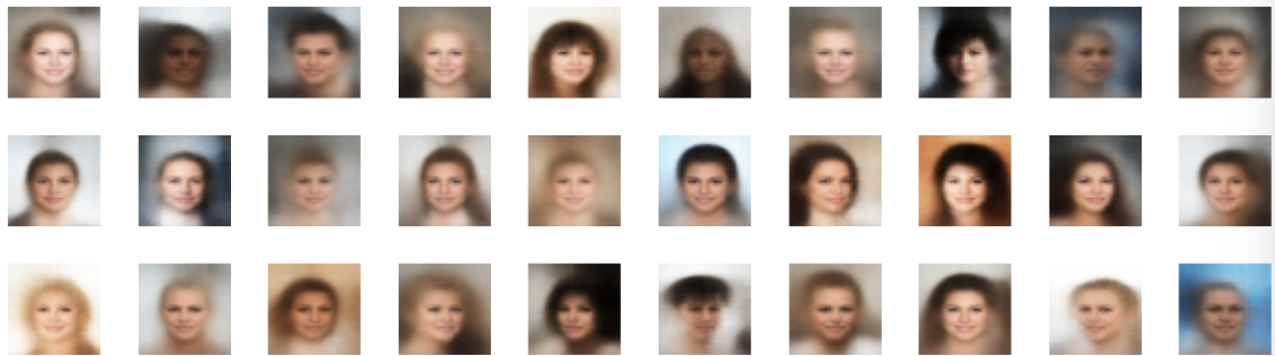
이제 디코더를 활용해서 새로운 얼굴을 생성해보겠습니다. 표준 정규분포에서 잠재 공간의 일부 포인트를 랜덤으로 샘플링해줍니다.

# 표준 정규 분포에서 잠재 공간의 일부 포인트를 샘플링합니다.

grid_width, grid_height = (10, 3)

z_sample = np.random.normal(size=(grid_width * grid_height, Z_DIM))

# 표준 정규 분포에서 잠재 공간의 일부 포인트를 샘플링합니다.

grid_width, grid_height = (10, 3)

z_sample = np.random.normal(size=(grid_width * grid_height, Z_DIM))

# 디코딩된 이미지의 그리기

fig = plt.figure(figsize=(18, 5))

fig.subplots_adjust(hspace=0.4, wspace=0.4)

# 얼굴 그리드 출력

for i in range(grid_width * grid_height):

    ax = fig.add_subplot(grid_height, grid_width, i + 1)

    ax.axis("off")

    ax.imshow(reconstructions[i, :, :])

 

생성된 이미지는 원본과는 다른 다양한 형태를보이고 있음을 알 수 있습니다.

 

 

이번에는 레이블을 조작해서 이미지를 의도한 대로 조작해보겠습니다. 

 

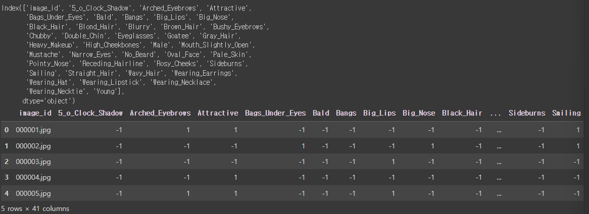
먼저 데이터의 레이블을 확인해봅니다.

# 레이블 데이터셋 로드

attributes = pd.read_csv("./list_attr_celeba.csv")

print(attributes.columns)

attributes.head()

 

총 40개의 attributes의 목록과 이진화 되어 있는 것을 알 수 있습니다.

 

이제 레이블이 부착된 얼굴 이미지를 로드해서, 특정 속성을 기준으로 데이터를 준비해보겠습니다. 예시는 금발(Blond_Hair)입니다.

# 레이블이 부착된 얼굴 데이터 로드

LABEL = "Blond_Hair"  # <- 이 레이블 설정

labelled_test = utils.image_dataset_from_directory(

    "./img_align_celeba",

    labels=attributes[LABEL].tolist(),

    color_mode="rgb",

    image_size=(IMAGE_SIZE, IMAGE_SIZE),

    batch_size=BATCH_SIZE,

    shuffle=True,

    seed=42,

    validation_split=0.2,

    subset="validation",

    interpolation="bilinear",

)

labelled = labelled_test.map(lambda x, y: (preprocess(x), y))

 

Blond_Hair라는 Attributes는 2개의 클래스 (1 또는 -1)이 있음을 확인하였고, 또한, 40,519개의 데이터가 Validation으로 활용되고 있음을 알 수 있습니다.

 

주어진 레이블에 해당하는 속성 벡터를 찾는 함수를 활용해 줍니다.

# 속성 벡터 찾기

attribute_vec = get_vector_from_label(labelled, vae, Z_DIM, LABEL)

 

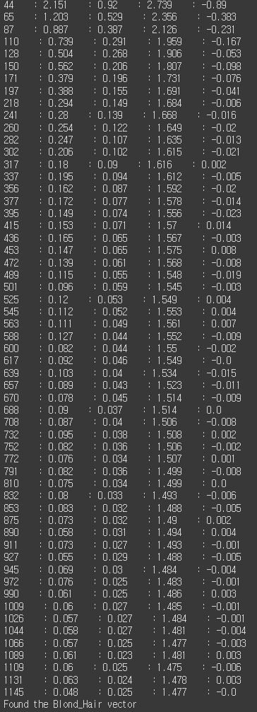
결과는 아래와 같습니다. 각 순서의 데이터가 해당 attributes에 대한 z vector 값은 다음과 같이 다름을 알 수 있습니다. 

기존 attributes에서는 1 또는 -1 (1 : 금발, -1 : 금발 아님) 이었으나, 이를 잠재 공간에서 z 벡터로 매핑하니 연속형 값으로 나옴을 알 수 있습니다.

 

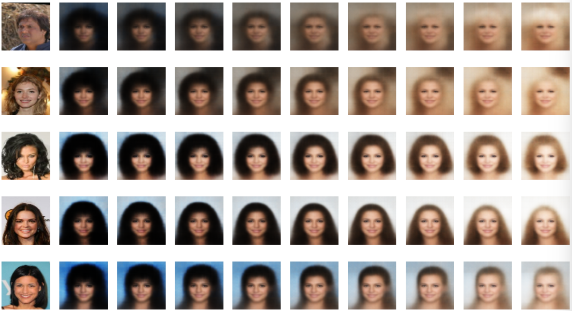
그렇다면 이미지에 Blond_Hair에 해당하는 잠재 벡터를 다른 값으로 더해보겠습니다. 왼쪽부터 작은 값을, 그리고 오른쪽으로 갈수록 큰 값이 더해지게 됩니다. 결과는 오른쪽으로 갈수록 점차 금발화가 되어감을 알 수 있으며, 또한 금발이라는 특성과 해당 사람의 형상이 연계되어 있어 형상 또한 같이 변함을 알 수 있습니다.

 

# 이미지에 벡터 추가

add_vector_to_images(labelled, vae, attribute_vec)