
이번에 알아볼 모델은 로지스틱 회귀(Logistic Regression)입니다.
로지스틱 회귀는 선형 회귀 방식을 분류에 적용한 알고리즘을 말합니다.
(이때, 회귀가 선형인가 비선형인가 하는 구분은 독립 변수가 아닌, 가중치(Weight) 변수가 선형인지 아닌지를 따릅니다.)
1. 로지스틱 회귀(Logistic Regression)란?
- 로지스틱 회귀는 로지스틱 함수(시그모이드(Sigmoid) 함수라고도 불립니다)를 사용하는 알고리즘으로, 분류(Classification) 문제를 다루는데 사용되는 알고리즘 중 하나입니다.
* 로지스틱(Logistic) 함수 ( 시그모이드(Sigmoid) 함수 라고도 불립니다)는 아래와 같습니다.
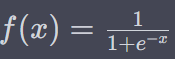
* 이 함수에서 e는 자연 로그의 밑(약 2.71828)이며, x는 입력변수르 의미합니다. 해당 함수는 입력 변수를 받아 0과 1사이의 확률로 변환하는데 사용되는 함수이기에, 0 또는 1로 분류하는 이진 분류문제에 많이 사용됩니다.
* 즉, 어떤 값들(X)이 해당 함수로 입력값으로 들어오게 되면, 0과 1사이의 값을 도출하며 이를 이벤트가 발생(0과 1 중 1이 발생) 확률로 해석하여 더 가까운 클래스로 예측하는 방법을 말합니다.
- 로지스틱 회귀 모델은 주어진 입력 변수와 파라미터를 사용하여 예측을 수행하고, 시그모이드 함수를 통해 확률값을 계산합니다.
* (일반적으로) 이때 계산된 값이 0.5보다 크면 "1"로 분류하고, 이보다 작으면 "0"으로 분류합니다. 이로 인해 이진 분류에 많이 사용됩니다.
* 해당 함수를 확장하여 다중 클래스 분류(Multiclass Classification)에 확장하여 사용되기도 합니다.
아래는 임의로 생성된 데이터를 활용하여 파이썬 코드로 선형 회귀와 로지스틱 회귀를 비교해보겠습니다.
이때 생성된 데이터는 (x,y) 값을 가지고 있으며, x는 실수 / y는 0 또는 1의 값을 가지는 데이터 입니다.
|
1
2
3
4
5
6
7
8
9
10
11
12
13
14
15
16
17
18
19
20
21
22
23
24
25
26
27
28
29
30
31
32
|
import numpy as np
import matplotlib.pyplot as plt
from sklearn.datasets import make_classification
from sklearn.linear_model import LogisticRegression, LinearRegression
# 인위적으로 생성한 데이터
X, y = make_classification(n_samples=100, n_features=1, n_informative=1, n_redundant=0, n_clusters_per_class=1, random_state=42)
# 로지스틱 회귀 모델 훈련
logreg = LogisticRegression()
logreg.fit(X, y)
# 단순 선형 회귀 모델 훈련
linreg = LinearRegression()
linreg.fit(X, y)
# 예측을 위한 X 값 생성
x_range = np.linspace(X.min() - 0.5, X.max() + 0.5, 300)
y_pred_logreg = logreg.predict_proba(x_range.reshape(-1, 1))[:, 1]
y_pred_linreg = linreg.predict(x_range.reshape(-1, 1))
# 시각화
plt.figure(figsize=(10, 5))
plt.scatter(X, y, label='Data', color='blue')
plt.plot(x_range, y_pred_logreg, label='Logistic Regression', color='green', linewidth=2)
plt.plot(x_range, y_pred_linreg, label='Simple Linear Regression', color='red', linewidth=2)
plt.xlabel('X')
plt.ylabel('Y (0 or 1)')
plt.legend()
plt.title('Logistic vs Simple Linear')
plt.ylim(-.1, 1.1) # Y 축 범위 설정
plt.show()
|
cs |
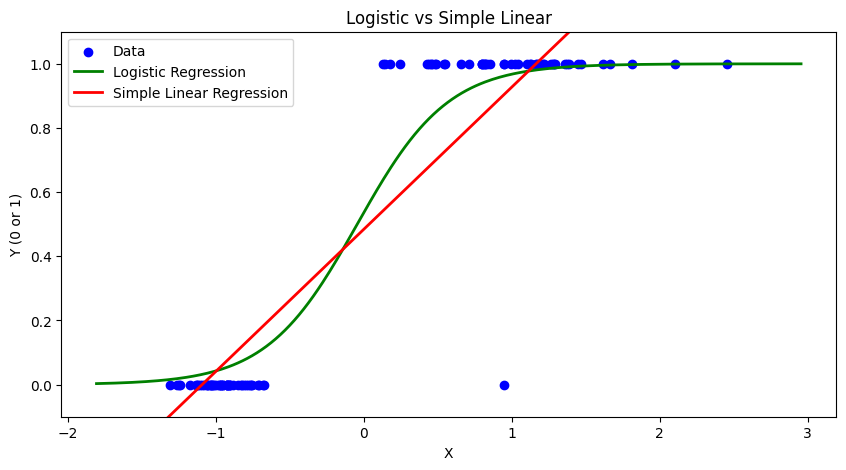
* 실제 자연 및 사회 현상에서도 위처럼 x의 값이 커지면 특정 이벤트가 발생하는 경우가 많은 데이터가 많은데요(ex. x는 종양의 크기, y는 암 발생 / x는 흡연기간, y는 암 발생 등)
* 이때, 위 빨간선처럼 단순 선형회귀를 통해 해당 현상을 예측하는 것보다는 초록색의 로지스틱 회귀를 통해 예측을 한다면 더 예측값이 정확해지는 것을 알 수 있습니다.
2. 유방암 데이터(Breast Cancer)를 활용한 로지스틱 회귀로 암 여부 진단
- 이번에는 파이썬 코딩을 통해 유방암 데이터 세트를 이용해 로지스틱 회귀로 암 여부를 진단해보겠습니다.
* 먼저, 데이터 처리와 시각화를 위해 pandas와 pyplot 라이브러리를 임포트하고, scikit learn에 내재된 breast cancer 데이터를 불러오고 이를 'cancer' 라는 개체명으로 저장합니다.
|
1
2
3
4
5
6
7
|
import pandas as pd
import matplotlib.pyplot as plt
from sklearn.datasets import load_breast_cancer
from sklearn.linear_model import LogisticRegression
cancer = load_breast_cancer()
|
cs |
* 선형 회귀 계열의 로지스틱 회귀는 데이터의 정규 분포도에 따라 예측 성능에 영향을 받을 수 있으므로, StandardScaler로 features(X)를 정규화해주고, 학습 및 테스트를 위해 데이터를 train set과 test set으로 나누어줍니다.
|
1
2
3
4
5
6
7
8
|
from sklearn.preprocessing import StandardScaler
from sklearn.model_selection import train_test_split
# StandardScaler( )로 평균이 0, 분산 1로 데이터 분포도 변환
scaler = StandardScaler()
data_scaled = scaler.fit_transform(cancer.data)
X_train , X_test, y_train , y_test = train_test_split(data_scaled, cancer.target, test_size=0.3, random_state=0)
|
cs |
*이후, 학습결과를 척도를 accuarcy와 roc_auc 스코어로 평가하기위해 해당 라이브러리를 임포트하고, 로지스틱 회귀를 이용해 학습 및 테스트를 수행합니다.
|
1
2
3
4
5
6
7
8
9
10
|
from sklearn.metrics import accuracy_score, roc_auc_score
# 로지스틱 회귀를 이용하여 학습 및 예측 수행.
lr_clf = LogisticRegression()
lr_clf.fit(X_train, y_train)
lr_preds = lr_clf.predict(X_test)
# accuracy와 roc_auc 측정
print('accuracy: {:0.3f}'.format(accuracy_score(y_test, lr_preds)))
print('roc_auc: {:0.3f}'.format(roc_auc_score(y_test , lr_preds)))
|
cs |
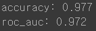
* 결과는 97.7%의 정확도와 0.972의 roc_auc 스코어가 나오게 되었습니다.
* 해당 결과를 시각화 해보겠습니다. 1) Confusion Matrix와 2) ROC-AUC 그래프 입니다.
1) Confusion Matrix)
|
1
2
3
4
5
6
7
8
9
10
11
12
13
14
15
16
17
18
19
|
# Confusion Matrix 계산
from sklearn.metrics import confusion_matrix
conf_matrix = confusion_matrix(y_test, lr_preds)
# Confusion Matrix 시각화
plt.figure(figsize=(8, 6))
plt.matshow(conf_matrix, cmap=plt.cm.Blues, fignum=1)
plt.title('Confusion Matrix')
plt.colorbar()
plt.xticks([0, 1], ['Predicted 0', 'Predicted 1'])
plt.yticks([0, 1], ['True 0', 'True 1'])
for i in range(2):
for j in range(2):
plt.text(j, i, str(conf_matrix[i, j]), ha='center', va='center', color='black', fontsize=20)
plt.xlabel('Predicted')
plt.ylabel('True')
plt.show()
|
cs |
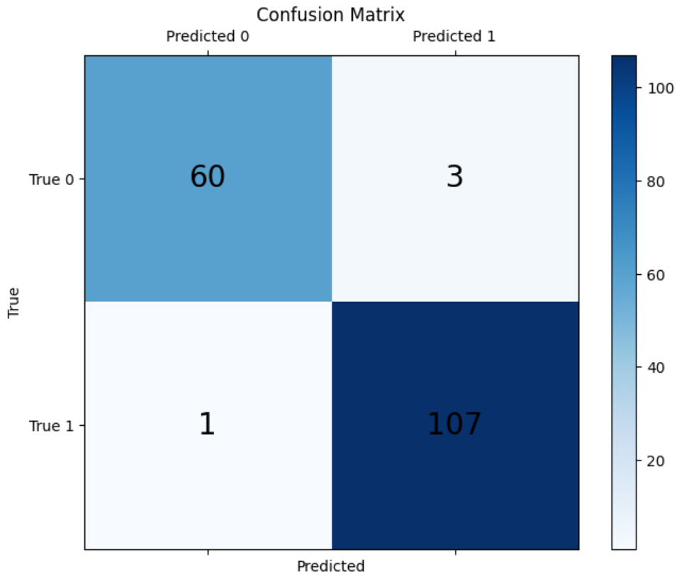
* 총 171개의 테스트 데이터 중 단 4개의 데이터를 제외한 167개의 데이터를 정확하게 예측했습니다.
Accuracy = 97.7% (= 167/171 * 100)
* 이번에는 ROC Curve 및 AUC를 시각화 해보겠습니다.
|
1
2
3
4
5
6
7
8
9
10
11
12
13
14
15
16
17
18
|
# ROC Curve 및 AUC 시각화
from sklearn.metrics import roc_curve, auc, roc_auc_score
fpr, tpr, thresholds = roc_curve(y_test, lr_clf.predict_proba(X_test)[:, 1])
roc_auc = auc(fpr, tpr)
plt.figure(figsize=(8, 6))
plt.plot(fpr, tpr, color='darkorange', lw=2, label='ROC curve (area = {:0.3f})'.format(roc_auc))
plt.plot([0, 1], [0, 1], color='navy', lw=2, linestyle='--')
plt.xlim([0.0, 1.0])
plt.ylim([0.0, 1.05])
plt.xlabel('False Positive Rate')
plt.ylabel('True Positive Rate')
plt.title('Receiver Operating Characteristic (ROC)')
plt.show()
# ROC AUC Score 출력
print('ROC AUC Score: {:0.3f}'.format(roc_auc_score(y_test , lr_preds)))
|
cs |

위와 같이 이진 분류에서 많이 사용되는 분류 모형 중 하나인 로지스틱 회귀에 대해서 알아보았습니다.
'머신러닝 with Python' 카테고리의 다른 글
| [머신러닝 with 파이썬] Pycaret이란? Pycaret을 활용한 머신러닝 (0) | 2023.09.24 |
|---|---|
| [머신러닝 with 파이썬] 회귀 트리(Regression Tree) (0) | 2023.09.23 |
| [머신러닝 with 파이썬] 경사하강법(Gradient Descent) / 확률적 경사하강법(Stochastic Gradient Descent) (0) | 2023.09.21 |
| [머신러닝 with Python] 선형회귀(Linear Regression) / 당뇨병(Diabetes) 데이터 활용 / EDA 시각화 포함 (0) | 2023.09.19 |
| [머신러닝 with Python] 선형회귀(Linear Regression) / 최소제곱법(Least Square Methods) (1) (0) | 2023.09.18 |


댓글